
언빌리버블티
[ML Study] Pima Indians Diabetes Classification : sklearn Decision Tree 를 이용한 분류 모델 본문
멋쟁이사자처럼kdt/천리길도한걸음씩👣
[ML Study] Pima Indians Diabetes Classification : sklearn Decision Tree 를 이용한 분류 모델
나는 정은 2022. 11. 2. 01:35멋쟁이 사자처럼 천리길도 한걸음씩 ML 스터디
week 5
Pima Indians Diabetes Classification
: sklearn 결정 트리를 이용한 분류
데이터 셋 출처
https://www.kaggle.com/uciml/pima-indians-diabetes-database
https://scikit-learn.org/stable/modules/generated/sklearn.datasets.load_diabetes.html
Columns 설명
- Pregnancies : 임신 횟수
- Glucose : 2시간 동안의 경구 포도당 내성 검사에서 혈장 포도당 농도
- BloodPressure : 이완기 혈압 (mm Hg)
- SkinThickness : 삼두근 피부 주름 두께 (mm) -> 체지방 추정용
- Insulin : 2시간 혈청 인슐린 (mu U / ml)
- BMI : 체질량 지수 (체중kg / 키(m)^2)
- DiabetesPedigreeFunction : 당뇨병 혈통 기능
- Age : 나이
- Outcome : 768개 중에 268개의 결과 클래스 변수(0 또는 1)는 1이고 나머지는 0
0. 라이브러리 로드
import numpy as np
import pandas as pd
import seaborn as sns
import matplotlib.pyplot as plt
import koreanize_matplotlib
from sklearn.model_selection import train_test_split
from sklearn.tree import plot_tree
from sklearn.metrics import accuracy_score
1. Data Load 및 EDA
a. 데이터 크기
df_pima = pd.read_csv("http://bit.ly/data-diabetes-csv")
df_pima.shape(768, 9)b. 데이터 확인
df_pima.info()<class 'pandas.core.frame.DataFrame'>
RangeIndex: 768 entries, 0 to 767
Data columns (total 9 columns):
# Column Non-Null Count Dtype
--- ------ -------------- -----
0 Pregnancies 768 non-null int64
1 Glucose 768 non-null int64
2 BloodPressure 768 non-null int64
3 SkinThickness 768 non-null int64
4 Insulin 768 non-null int64
5 BMI 768 non-null float64
6 DiabetesPedigreeFunction 768 non-null float64
7 Age 768 non-null int64
8 Outcome 768 non-null int64
dtypes: float64(2), int64(7)
memory usage: 54.1 KB- null 값은 존재하지 않음
c. 데이터 분포 확인
df_pima.hist(figsize=(12,10), bins=50)
plt.show()
- SkinThickness와 Insulin, BMI에 이상치가 있다는 사실을 확인 할 수 있다.
- 전처리를 하지 않은 상태에서 모델 성능 평가를해보고, 이후 하이퍼파라미터 튜닝을 진행하며 차이 비교
- 지도 학습의 경우 기본적으로 문제의 답을 제시하고 있음, pima 데이터에서는 Outcome이 답에 해당함
2. 모델 학습
a. 데이터셋 나누기 train - test
feature_names = df_pima.columns.to_list()
feature_names.remove("Outcome")
feature_names
['Pregnancies','Glucose','BloodPressure','SkinThickness',
'Insulin', 'BMI', 'DiabetesPedigreeFunction', 'Age']label_name = "Outcome"X = df_pima[feature_names]
y = df_pima[label_name]from sklearn.model_selection import train_test_split
X_train, X_test, y_train, y_test = train_test_split(X, y, test_size=0.2, random_state=42)
X_train.shape, y_train.shape, X_test.shape, y_test.shape((614, 8), (614,), (154, 8), (154,))- train_test_split()
- arrays : 분할시킬 데이터
- test_size: 테스트 셋의 비율, default = 0.25
- train_size: 학습 데이터 셋의 비율, defalut = 1-test_size
- random_state : 고정할 seed값
- shuffle: 기존 데이터를 나누기 전에 순서를 섞을것인지, default = True
- stratify: 지정한 데이터의 비율을 유지, 분류 문제의 경우 해당 옵션이 성능에 영향이 있다고는 함
b. 결정 트리 학습법
CART (Classificaton and Regression Trees) 알고리즘
- 어떤 항목에 대한 관측값과 목표값을 연결 시켜주는 예측 모델로서 사용
- 분류 트리: 목표 변수가 유한한 수의 값
- 회귀 트리: 목표 변수가 연속하는 값
- 트리 최상단에는 가장 중요한 질문이 옴
- 결과를 해석(화이트박스 모델)하고 이해하기 쉬움
- 수치 / 범주형 자료에 모두 적용 가능
- 지니 불순도를 이용
# 사이킷런의 의사결정트리 알고리즘 load
from sklearn.tree import DecisionTreeClassifier

model = DecisionTreeClassifier(random_state=42)
model
DecisionTreeClassifier() 주요 파라미터
-
- criterion: 가지의 분할의 품질을 측정하는 방식
- max_depth: 트리의 최대 깊이
- min_samples_split : 내부 노드를 분할하는 데 필요한 최소 샘플 수
- min_samples_leaf: 리프 노드에 있어야 하는 최소 샘플 수
- max_leaf_nodes: 리프 노드 숫자의 제한치
- random_state: 추정기의 무작위성을 제어
c. 모델 학습 및 예측 평가
# Train
model.fit(X_train, y_train)

# Predict Test
y_predict = model.predict(X_test)
y_predictarray([1, 0, 0, 0, 0, 0, 0, 0, 0, 1, 0, 1, 1, 1, 0, 0, 0, 0, 1, 0, 1, 0,
0, 0, 0, 1, 0, 0, 0, 0, 1, 1, 1, 1, 0, 1, 1, 0, 0, 1, 0, 1, 1, 1,
0, 1, 1, 0, 0, 1, 0, 1, 1, 0, 0, 0, 0, 0, 0, 1, 1, 0, 1, 0, 0, 0,
0, 1, 0, 1, 1, 0, 0, 0, 0, 1, 0, 0, 0, 0, 1, 0, 0, 1, 1, 1, 1, 1,
1, 0, 0, 0, 0, 1, 1, 0, 1, 0, 1, 0, 1, 0, 1, 0, 1, 0, 0, 1, 0, 1,
0, 0, 0, 1, 1, 1, 1, 0, 0, 1, 0, 0, 0, 0, 0, 1, 1, 1, 1, 1, 1, 1,
0, 0, 1, 1, 0, 1, 1, 0, 0, 0, 0, 0, 0, 0, 0, 0, 0, 1, 0, 1, 0, 0],
dtype=int64)# Accuracy 출력
# (y_test == y_predict).mean() 과 같다.
from sklearn.metrics import accuracy_score
accuracy_score(y_test, y_predict)# 모델에서 score를 호출해 정확도를 구할 수도 있다.
model.score(X_test, y_test)0.7467532467532467d. Feature importance 분석
I. plot_tree를 이용해 DT 알고리즘을 시각화할 수 있다.
from sklearn.tree import plot_tree

plt.figure(figsize=(20,20))
plot_tree(model, max_depth=3, feature_names=feature_names, filled=True, fontsize = 16)
plt.show()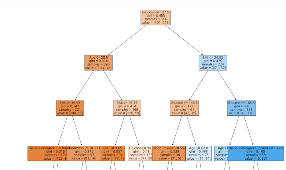
- 결정 트리의 최상위에 Glucose가 온 것을 확인 할 수 있다.
- 결정 트리의 최상단에는 가장 중요한 feature가 오므로 제일 중요한 변수는 glucose
II. Feautre Importances 추출하기
- 모델에서 바로 변수 중요도를 추출할 수 있다.
model.feature_importances_array([0.05748153, 0.31422474, 0.14767907, 0.06116378, 0.06625279,
0.17070035, 0.08328237, 0.09921536])sns.barplot(x=model.feature_importances_, y=model.feature_names_in_)
plt.show()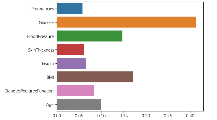
3. Decision Tree Model 하이퍼 파라미터 조정
- feature의 개수 또는 최대 깊이를 제한하여 모델을 재구성하고 성능을 평가
- 맨 처음 accuracy = 0.7467
a. 결정 트리 모델의 최대 높이 = 4 & 고려 특성 비율 = 0.8 로 파라미터 조정
model = DecisionTreeClassifier(random_state=42, max_depth=4, max_features=0.8)
model.fit(X_train, y_train)
y_pre_max4 = model.predict(X_test)
y_pre_max4array([0, 0, 0, 0, 0, 0, 0, 1, 0, 0, 0, 1, 0, 1, 0, 0, 0, 0, 1, 0, 0, 0,
0, 0, 0, 1, 0, 0, 0, 1, 0, 0, 1, 1, 1, 1, 1, 1, 0, 1, 0, 1, 1, 0,
0, 0, 1, 0, 0, 1, 0, 1, 0, 0, 0, 0, 0, 0, 0, 1, 0, 0, 0, 1, 0, 0,
0, 0, 0, 1, 1, 0, 0, 0, 0, 0, 0, 0, 0, 0, 1, 0, 0, 0, 0, 1, 0, 1,
0, 0, 0, 0, 0, 0, 0, 0, 0, 0, 0, 0, 1, 0, 1, 0, 1, 0, 0, 1, 0, 1,
0, 1, 0, 1, 0, 0, 1, 0, 0, 0, 0, 0, 0, 0, 0, 0, 0, 1, 1, 1, 1, 1,
0, 0, 1, 0, 0, 1, 1, 0, 0, 0, 0, 0, 0, 0, 1, 0, 0, 1, 0, 0, 0, 1],
dtype=int64)accuracy_score(y_test, y_pre_max4)0.7597402597402597b. Feature Engineering
- Garbage In - Garbage Out : 잘 전처리된 데이터를 사용하면 좋은 성능이 나온다는 의미
- 실제 모델을 생성하기 이전에 EDA를 통해, 데이터를 분석하고 전처리하는 과정이 중요하다.
I. 수치형 변수 -> 범주형 변수로 만들기
sns.countplot(data=df_pima,x='Pregnancies')plt.figure(figsize=(15,6))
sns.countplot(data=df_pima, x="Pregnancies", hue="Outcome")
plt.show()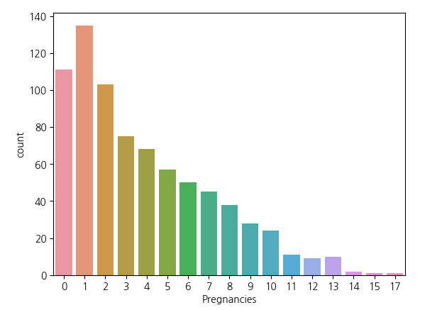
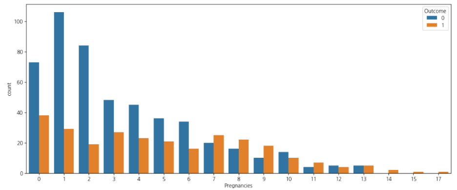
- Pima 인디언 데이터 셋에서 Pregnancies의 경우 3회 미만인 경우가 대부분이다.
- 0 ~ 17까지 수치형 범주지만, 범주형 변주로 바꾸는 피쳐 엔지니어링을 진행한다.
- 임신 횟수를 기준으로 6회 이상인지 아닌지를 표현하는 데이터로 변환
df_pima["Pregnancies_high"] = df_pima["Pregnancies"] > 6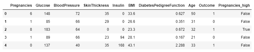
model = DecisionTreeClassifier(random_state=42, max_depth=4, max_features=0.8)
model.fit(X_train, y_train)
y_pre_max4_Pre_high = model.predict(X_test)
accuracy_score(y_test, y_pre_max4_Pre_high)0.7727272727272727- 성능이 처음보다 3점 정도 향상되었음.
II. 결측치 처리하기
- Insulin의 결측치 데이터를 처리
# Outcome을 기준으로, Insulin의 값을 구분해 KDE와 시각화
sns.histplot(data = df2, x ="Insulin", hue = "Outcome", kde = True)
plt.show()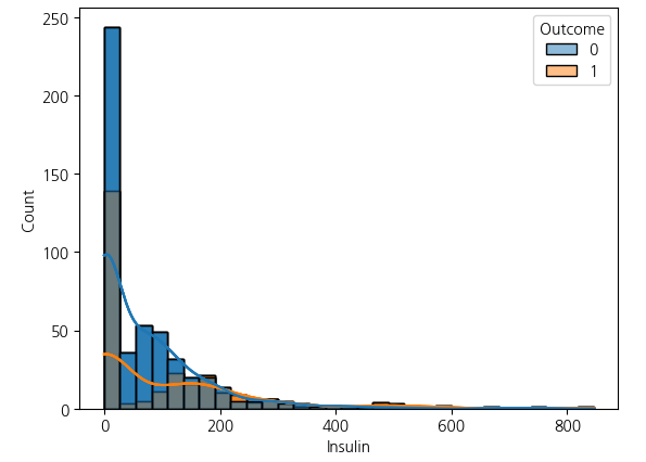
- seaborn hist에서 kde(밀도 추정)을하면 해당 레이블의 밀도를 확인 가능하다.
- Insulin 항목에서 약 48%의 결측치가 존재함
- 결측치를 해결하는 방법은 여러가지가 존재하지만, 중앙값으로 대체하는 방식과 평균값으로 보완 두 가지 방식으로 진행
II_a. Insulin 데이터 결측치 처리하기 - 중앙값으로 채우기
df_pima["Insulin_filled"] = df_pima["Insulin"].replace(0,np.nan)
Insulin_median = df_pima.groupby("Outcome")["Insulin_filled"].median()
Insulin_median
Outcome
0 102.5
1 169.5
Name: Insulin_nan, dtype: float64df2["Insulin_fill"] = df2["Insulin_nan"]
df_pima.loc[(~df_pima["Outcome"])&df_pima["Insulin_filled"].isnull(), "Insulin_filled"] = Insulin_median[0]
df_pima.loc[(df_pima["Outcome"])&df_pima["Insulin_filled"].isnull(), "Insulin_filled"] = Insulin_median[1]model = DecisionTreeClassifier(random_state=42, max_depth=4, max_features=0.8)
model.fit(X_train, y_train)
y_pre_max4_50_per = model.predict(X_test)
accuracy_score(y_test, y_pre_max4_50_per)0.8961038961038961- 성능이 눈에 띄게 오른 것을 확인할 수 있었다.
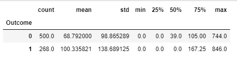
II_b. Insulin 데이터 결측치 처리하기 - 평균값으로 채우기
df_pima["Insulin_filled"] = df_pima["Insulin"].replace(0,np.nan)
Insulin_mean = df_pima.groupby("Outcome")["Insulin"].mean()
Insulin_mean
Outcome
0 68.792000
1 100.335821
Name: Insulin, dtype: float64df2["Insulin_fill_mean"] = df2["Insulin_nan"]
df_pima.loc[(~df_pima["Outcome"])&df_pima["Insulin_filled"].isnull(), "Insulin_filled"] = Insulin_mean[0]
df_pima.loc[(df_pima["Outcome"])&df_pima["Insulin_filled"].isnull(), "Insulin_filled"] = Insulin_mean[1]model = DecisionTreeClassifier(random_state=42, max_depth=4, max_features=0.8)
model.fit(X_train, y_train)
y_pre_max4_mean = model.predict(X_test)
accuracy_score(y_test, y_pre_max4_mean)0.8506493506493507- Insulin의 결측치를 처리하기 이전(0.77)보다는 약 8점 정도의 성능 향상이 있지만, 중앙값으로 대체한 경우(0.88)보다는 성능이 3점 정도 낮음
III. 이상치 분석하기
- 평균치를 처리한 데이터로 이상치가 있는지 탐색하기
# 인슐린의 결측치를 평균값으로 처리한 경우의 이상치를 시각화
plt.figure(figsize=(15, 2))
sns.boxplot(df_pima["Insulin_filled"])
plt.title("결측치를 평균값으로 처리한 경우");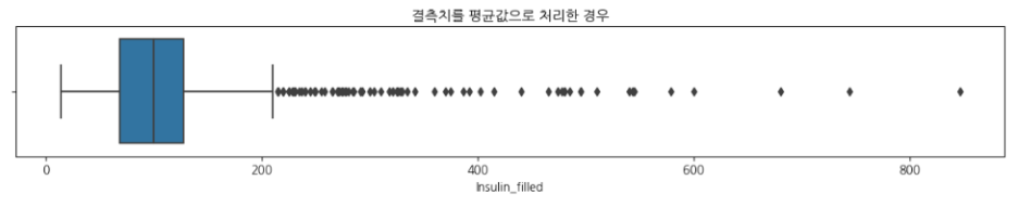
# 통계값
df_pima["Insulin_filled"].describe()
count 768.000000
mean 118.967780
std 93.557899
min 14.000000
25% 68.792000
50% 100.000000
75% 127.250000
max 846.000000
Name: Insulin_filled, dtype: float64# KDE로 이상치 처리 이전의 값 시각화
df_pima["Insulin_filled"].plot(kind="kde")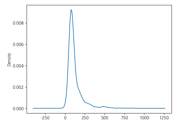
- 결측치를 채워줬지만 이상치가 끼어있는 문제가 있다.
- 75% 이상의 데이터를 모두 평균으로 대체해주고 모델을 생성
desc = df_pima["Insulin_filled"].describe()
df_pima[df_pima["Insulin_filled"] > desc["75%"]]

df_pima.loc[(~df_pima["Outcome"])&(df_pima["Insulin_filled"] > desc["75%"]), "Insulin_filled"] = Insulin_mean[0]
df_pima.loc[(df_pima["Outcome"]==1)&(df_pima["Insulin_filled"] > desc["75%"]), "Insulin_filled"] = Insulin_mean[1]
# 이상치 처리 후 값을 시각화
plt.figure(figsize=(15, 2))
sns.boxplot(df_pima["Insulin_filled"])
plt.title("이상치 처리 후")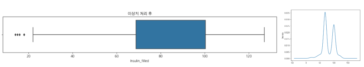
IV. 이상치 제거한 데이터셋 모델 생성 및 평가
model.fit(X_train, y_train)
y_pre_max4_mean_out = model.predict(X_test)
y_pre_max4_mean_out

accuracy_score(y_test, y_pre_max4_mean_out)0.8441558441558441- 이상치를 처리한 후에 성능이 조금 떨어졌다.
- 통계를 기반으로하는 이상치 처리는 위험할 수도 있으므로 해당 데이터 변수들의 의미와 도메인을 이해하고 원인을 파악하고 처리해야 한다.
Comments